Induced earthquake mechanisms

Induced earthquake mechanism - Poroelasticity

Poroelasticity is a field in materials science and mechanics that studies the
interaction between fluid flow and solids deformation with a linear porous medium. (wiki)

We start from the solid energy equation [1]

[1]

Oliver Coussy 2010. Mechanics and Physics of Porous Solids, WILEY

\[\sigma\text{d} \epsilon - \varphi \text{d} p + s_{ij}\text{d} e_{ij} - \text{d} \eta_S = 0\]

from here, we then have:

\[\begin{split}\begin{align} \frac{\partial \eta_s}{\partial \epsilon} &= \sigma \\ \frac{\partial \eta_S}{\partial p} & = -\varphi \\ \frac{\partial \eta_S}{\partial e_{ij}} &= s_{ij} \end{align}\end{split}\]

Previous equation could also be rewritten as below:

Warning

Readers are suggested to refer to the textbook and please kindly let me know if you have any idea on the formula transition

\[\eta_S = \frac{1}{2}K\epsilon^2+Ge_{ij}\cdot e_{ij}-\alpha\epsilon p-\frac{1}{2}\frac{P^2}{N}\]

therefore, we have:

\[\begin{split}\begin {align} \sigma &= \frac{\partial \eta_S}{\partial \epsilon} = K\epsilon - \alpha p\\ \varphi &= \frac{\partial \eta_S}{\partial p} = \alpha \epsilon + \frac{p}{N}\\ s_{ij} &= 2G\cdot e_{ij} \end{align}\end{split}\]

\(K\) is bulk modulus when there is no pore pressure.

\(\varphi = \phi-\phi_0\) is the change of Lagrangian porosity, where \(\phi_0\) is the initial porosity before deformation.

\(\alpha\), also named Biot coefficient, is the ratio of porosity change over volumetric strain when pore pressure is 0. The relationship among volometric strain \(\epsilon\), solid volumetric strain \(\epsilon_S\) and \(\varphi\) \(\epsilon = (1-\phi_0)\epsilon_S + \varphi\). A high \(\alpha\) value means higher solid stiffness (larger \(K\)).

\(N\) is the poroelastic modulus measured by the ratio between the porosity change \(\varphi\) and the pore-pressure when volumetric strain is zero.

Biot coefficient

As introduced in above section, here we further derive the relationship between \(\alpha\),:math:K and \(K_S\).

Note

Jacketed condition: No pore pressure in pores. Unjacketed condition: the pore pressure equals to the stress applied.

In the Jacketed condition, we can measure the jacketed bulk modulus \(K\). In the UNjacketed condition, we then have

\[K\epsilon -\alpha p = p\]

which leads to \(\epsilon = \frac{p(1+\alpha)}{K}\).

For the solid material, we then have:

\[\epsilon_S = \frac{p}{K_S}\]

In the Jacketed conditon, we have \(\epsilon = \epsilon_S\), which leads to:

\[\frac{p}{K_S} = \frac{p(1+\alpha)}{K}\]

we then have \(\alpha = 1-\frac{K}{K_S}\)

How poroelasticity induce earthquakes

Warning

This part is based on the knowledge of Mohr circle.

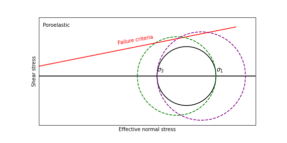
Schematic plot showing the effects of poroelasticity

The increase of \(\sigma_1\) or the decrease of \(\sigma_3\) could both bring the fault closer to failure.

The Biot modulus

For a porous solid, its Lagrangian porosity \(\phi\) is defined as the ratio of the volume of porous \(V_p\) and the total (bulk) volume \(V_b\). The fluid mass in pores is \(m_F=V_p\cdot \rho_F\), where \(\rho_F\) denotes fluid density. For a unit volume, the expression could be written as

\[\frac{m_F}{V_b} = \frac{V_p\cdot \rho_F}{V_b} = \phi\rho_F\]

The differential of fluid mass could be written as

\[\text{d}({\phi\rho_F}) = \phi\text{d}\rho_F + \rho_F\text{d}\phi\]

and further transformed into

\[\frac{\text{d}({\phi\rho_F})}{\rho_F} = \phi\frac{\text{d}\rho_F}{\rho_F} +\text{d}\phi\]

As introduced in the poroelasticity mechanism, the porosity constitutive equation is

\[\phi = -\frac{\partial\eta_S}{\partial p} = \alpha \epsilon + \frac{p}{N}\]

therefore

\[\text{d}{\phi} = \alpha \text{d}\epsilon + \frac{\text{d}p}{N}\]

on the same time, the bulk modulus of fluid is defined as

\[K_F = \rho_F \frac{\text{d}p}{\text{d}\rho_F}\]

which leads to

\[\frac{\text{d}\rho_F}{\rho_F} = \frac{\text{d}p}{K_F}\]

we then get

\[\begin{split}\begin{align} \frac{\text{d}({\phi\rho_F})}{\rho_F} &= \phi\frac{\text{d}p}{K_F} + \alpha\text{d}\epsilon + \frac{\text{d}p}{N}\\ \frac{\text{d}({\phi\rho_F})}{\rho_F} &= (\frac{1}{N}+\frac{\phi}{K_F}){\text{d}p} + \alpha\text{d}\epsilon \end{align}\end{split}\]

In real case, the porosity change is very small. Therefore, \(\phi \approx \phi_0\). The Biot modulus \(M^*\) is then defined as \(\frac{1}{M^*}=\frac{1}{N}+\frac{\phi_0}{K_F}\).

Induced earthquake mechanism - Fluid diffusion

The fluid diffusion flows two laws: 1) The Darcy’s law and 2) The mass reservation law.

Note

The Darcy’s law describes the relationship between the flux and the pressure drop: \(q = -\frac{k}{\mu}\nabla p\), where \(k\) is the permeability and \(\mu\) is the viscosity.

According to the mass reservation law, we then have:

\[\begin{split}\begin{align} \frac{d(\phi\rho_F)}{\text{d}t} + \nabla (\rho_F\cdot q) &= 0\\ \frac{d(\phi\rho_F)}{\text{d}t} - \nabla (\rho_F\cdot \frac{k}{\mu}\Delta p) &= 0\\ \frac{\rho_F}{\text{d}t}(\alpha\text{d}\epsilon+\frac{1}{M^*}\text{d}p) - \nabla (\rho_F\cdot \frac{k}{\mu}\nabla p) &= 0\\ \alpha\frac{\text{d}\epsilon}{\text{d}t}+\frac{1}{M^*}\frac{\text{d}p}{\text{d}t} - \frac{k}{\mu}\nabla^2 p &= 0\\ \frac{\text{d}p}{\text{d}t} &= \frac{kM^*}{\mu}\nabla^2p - \alpha M^*\frac{\text{d}\epsilon}{\text{d}t} \end{align}\end{split}\]

this is the diffusivity equation coupled with poroelasticity. The first part in the right of the equal symbol denotes the migrated fluid due to pressure difference, the second part corresponds to the volumetric strain due to the pore pressure.

Note

The diffusion coefficient \(D\) is defined as \(D=\frac{kM^*}{\mu}\)

Diffusion front

By ignoring the volumetric strain part, the diffusivity equation is simplified to

\[\frac{\partial p}{\partial t} = D\nabla p\]

in homogeneous 3D structure, assuming the injection pressure is initiated in a sphere with radius \(a\) and decays in the follow the pattern \(p_0e^{-i\omega t}\), the solution to the differential equation is

\[p(r,t) = p_0e^{-i\omega t}\frac{a}{r}exp\left[(i-1)(r-a)\sqrt{\frac{\omega}{2D}}\right]\]

where \(\omega\) is the angular frequency. The attenuation coefficient is \(sqrt{\frac{\omega}{2D}}\), which means higher frequency component decays faster. The attenuation slowness is \(1/\sqrt{\omega 2D}\)

If there is a earthquake occurred at (\(x_0\), \(t_0\)), we then consider the process that

\[\begin{split}p = \begin{cases} 0, \quad & t<0\\ p_0, \quad &0<t\leq t_0\\ 0, \quad &t>t_0 \end{cases}\end{split}\]

The power spectrum of this funtion is

\[4p_0^2t_0^2\frac{\sin(\omega t_0/2)}{\omega^2 t_0^2}\]

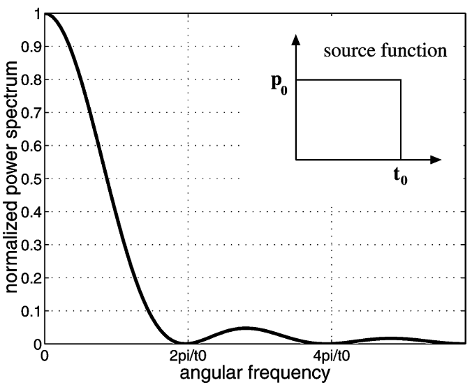
Power spectrum of a rectangle pulse (Shapiro et al., 2002)

It is reasonbale to consider the dominant frequency range is \(0-\frac{2\pi}{t_0}\) due to:

• The amplitude is much larger in the range \(0-\frac{2\pi}{t_0}\)

• The higher frequency compoent decays faster.

Consider an earthquake occurred in \((x_0,t_0)\), then it should occure before the relaxation time

\[t_0<=r_0\sqrt{t_0/(4\pi D)}\]

which leads to \(D\leq\frac{r_0^2}{4\pi t_0}\). Therefore, earthquakes related to fluid diffusion should be constrained by below relation

\[r<=\sqrt{4\pi D t}\]

We then could use this relationship to constrain the fluid diffusion coefficient.

How pore pressure induce earthquakes

Warning

This part is based on the knowledge of Mohr circle.

The fluid pressure exerts force towards every direction. Therefore, the pore-pressure will decrease both \(\sigma_1\) and \(\sigma_3\).

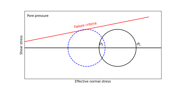
The increased pore pressure will decrease the effective normal stress and move the fault closer to failure.

The direct influence is the decrease of effctive normal stress. Therefore, the Mohr-circle is shifted leftwards (dashed blue), bring the fault plane closer to failure.

image_code

Induced earthquake mechanism - Aseismic slip

If a fault is slip-weakening, the accumulated slip tends to be released in the format of earthquakes. If a fault is slip-strengthening, the accumulated slip tends to be released in a aseismic way.

Rate- and state-dependent friction

\[\mu = \mu_0 + a*\ln\frac{v}{v_0} + b*\ln\frac{V_0\theta}{d_c}\]

where \(\mu_0\) is the static friction, \(v_0\) is the reference velocity that is in the level of plate convergence rate, \(v\) is velocity, \(d_c\) is the asperity contact characteristic length determined by experiment,

\(theta\) is the state variable, which satisfies \(\frac{\text{d}\theta}{\text{d}t}=1-\frac{v\theta}{d_c}\) from the expression, it is inferred that \(\theta\) increases with time with decreasing slope. The limit value will be achieved when \(1-\frac{v\theta}{d_c}=0\), the corresponding state variable value is \(\theta = \frac{d_c}{v}\).

Then we have:

\[\begin{split}\begin{align} \mu &= \mu_0 +a*\ln\frac{v}{v_0}-b*\ln\frac{v}{v_0}\\ &= \mu_0 + (a-b)\ln\frac{v}{v_0} \end{align}\end{split}\]

Here we discuss the scenario of increasing velocity, which means \(v>v_0\).

• If \(a-b>0\), \(\mu > \mu_0\), the characteristic is velocity stregthening.

• If \(a-b<0\), \(\mu < \mu_0\), the characteristic is velocity weakening.

Because the slip rate \(v\) and state variable \(\theta\) is invoved, this relationship is called rate- and state-dependent friction. The relationship is empirical and no full physcial meaning. We can still combine some understanding into the a, and b part. #. The a part could be considered as the fault opening process, where extra work needs to be done. #. The b part could be related to the fault healing process, for an opened fault plain, there are two effects:

• its asperities will decrease due to the slip, which will lead to a decrease friction coefficient

• the fault will heal itself with time goes on.

If the fault heals slowly, we then would expect a large b value. If the fault heals fast, we then would expect a small b value.